The increase was very rapid: from about 150 new cases on March 15 to nearly 30,000 cases on April 20 – an increase of a factor of nearly 200.
To control this unabated growth, measures such as night and weekend curfews were taken from April 21, which resulted in the imposition of a partial curfew, with markets, malls, restaurants etc. closed and large gatherings banned.
The number of cases peaked at around 38,000 on April 24, and then went down to 4,000 new cases on May 25.
What was the impact of the control strategy adopted by the state? Could it have been better to impose curfew earlier? We address and answer these questions below.
tomorrow model
We use the SUTRA model to analyze and study the progress of the pandemic in the state and simulate various strategies. The model has two parameters that control how fast the infection is spreading and its duration.
These are called reach and contact rates.
The parameter reach measures the fraction of the population on which the epidemic is currently active. It increases when the epidemic reaches new areas. It also increases when someone in a previously protected group living inside the “bubble” becomes infected.
The parameter contact rate measures how fast the epidemic is spreading in a population. It increases when people stop taking precautions, or a rapidly spreading mutant arrives. This comes down due to interventions like lockdown.
The model can estimate the value of the contact rate at any given time from the reported daily new infection data.
While it cannot calculate the value of access at a given point in time, it can estimate the change in the value of access between two given dates.
This allows the value of the access at any given time to be estimated relative to its value at a given point in time. By suitably varying the values of these two parameters, the alternative trajectory of the epidemic can be calculated.
Parameter values during March-May
The parameter values started increasing in the state from March 15 and doubled by the end of the month and the contact rate increased by 35% to 0.54.
This increase was due to the spread of the delta-variant as well as people not following the COVID-appropriate behaviour. The resulting increase was much faster as seen earlier.
Parameter values began to change again from April 21 – over the next two weeks, reach increased by 60%, but the contact rate dropped to 0.29, a drop of almost 50%. While the former was due to the epidemic spreading in the villages, the reduction in the contact rate was due to the containment measures.
Analysis
What would have happened if the contact rate did not come down at the end of April? The following plot shows that the 7-day average of daily new infections would have peaked at around 70,000 cases in the first week of May, which is twice the actual peak value.
By the end of April, state hospitals were finding it difficult to accommodate patients and oxygen supplies were running low, and a real catastrophe would have happened without preventive measures.
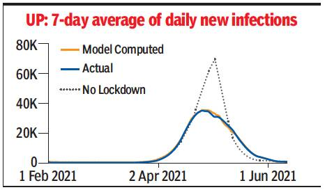
In the plot, the blue line indicates the trajectory of the 7-day moving average of daily transitions, the orange one shows the trajectory predicted by the model after estimating the parameters, and the dotted purple one shows the projected trajectory in a scenario where no Preventive measures are not taken. The seven-day average is used because there are weekly variations in the number of reported cases.
Could the case load have been significantly reduced by implementing the earlier measures?
To analyze this it is useful to understand the effect of change in contact rate.
When access is significantly increased, it makes it available for epidemics to infect large numbers of susceptible individuals.
If the contact rate is high at that time, then the infection starts spreading rapidly.
On the other hand, if the contact rate is low at that time, then the spread of infection is slow and the number drops to a much lower level.
The same is evident in the above plot, which shows a gradual decrease from the end of April, rather than a continuous increase, due to a significantly lower contact rate.
If the reduction in the contact rate occurs well after the expansion of reach, the epidemic has a chance to spread rapidly to the newly available susceptible population, and therefore the benefits of reduction in the contact rate are not so significant.
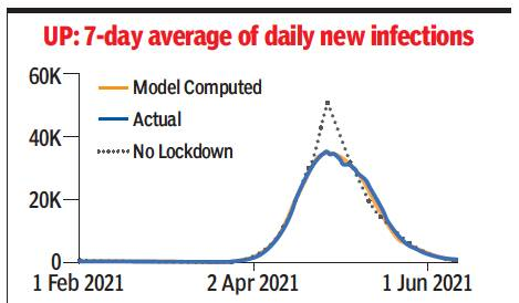
The next plot brings it out clearly: a week’s delay in implementing the measures in UP would have resulted in a peak of more than 50,000 for a 7-day average of daily infections by the end of April.
The above shows that earlier prevention measures would have helped greatly if they were taken in mid-March – however, no one could have predicted what would happen! The plot below shows the trajectory if the measures were taken a week ago.
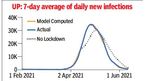
There is no significant gain here: the 7-day average of daily infections is around 30,000, just 5,000 less than the actual peak. The peak is also running late by about a week.
Conclusion
The analysis done with the help of formula model shows the success of containment measures taken in UP.
These helped avoid a major crisis as the epidemic was spreading in rural areas, which did not have good access to health facilities, and managed to control the pace of spread significantly.
The timing of the measures was also appropriate, even with a slight delay the case load could have been significantly higher and earlier measures would have helped only a little more.
The best part of the strategy was that, unlike many other states, it did not restrict everyone to their residences and allowed a large number of activities that did not disrupt the livelihood of a large section.
(The author is Professor of Computer Science and Engineering here It Kanpur)
.